The tidycensuskr package is designed for R users who want to work with South Korean census and administrative boundary data. It aims to provide an easy-to-use interface for population, housing, and socioeconomic statistics linked with geospatial boundaries.
Installation
You can install the released version of tidycensuskr from CRAN with:
# CRAN
install.packages("tidycensuskr")

# R-universe
install.packages("tidycensuskr", repos = "https://sigmafelix.r-universe.dev")
To install the development version, remotes::install_github() will suffice.
# Development version from GitHub
rlang::check_installed("remotes")
remotes::install_github("sigmafelix/tidycensuskr")
About the data
As of September 2025, this package contains two datasets: Census data (censuskor) and the corresponding geospatial data.
1. Census data
- Sigungu dataset of three census years (2010, 2015, 2020)
- The curated dataset is a long table (i.e., one row per district-year-variable)
anycensus()
- The function
anycensus()allows you to query census data for specific district or province codes and types of data (population, tax, mortality, economy, housing) for three census years (2010, 2015, 2020).
# loading Seoul population data
tidycensuskr::anycensus(codes = "Seoul", type = "population")
#> # A tibble: 25 × 17
#> year adm1 adm1_code adm2 adm2_code type all households_total…¹
#> <dbl> <chr> <dbl> <chr> <dbl> <chr> <dbl>
#> 1 2020 Seoul 11 Dobong-gu 11100 populat… 312878
#> 2 2020 Seoul 11 Dongdaemun-gu 11060 populat… 332796
#> 3 2020 Seoul 11 Dongjak-gu 11200 populat… 378749
#> 4 2020 Seoul 11 Eunpyeong-gu 11120 populat… 458777
#> 5 2020 Seoul 11 Gangbuk-gu 11090 populat… 295304
#> 6 2020 Seoul 11 Gangdong-gu 11250 populat… 440022
#> 7 2020 Seoul 11 Gangnam-gu 11230 populat… 509899
#> 8 2020 Seoul 11 Gangseo-gu 11160 populat… 564114
#> 9 2020 Seoul 11 Geumcheon-gu 11180 populat… 225594
#> 10 2020 Seoul 11 Guro-gu 11170 populat… 394733
#> # ℹ 15 more rows
#> # ℹ abbreviated name: ¹`all households_total_prs`
#> # ℹ 10 more variables: `all households_male_prs` <dbl>,
#> # `all households_female_prs` <dbl>, fertility_total_brt <dbl>,
#> # `fertility_15-19 (simulated)_bp1` <dbl>, `fertility_20-24_bp1` <dbl>,
#> # `fertility_25-29_bp1` <dbl>, `fertility_30-34_bp1` <dbl>,
#> # `fertility_35-39_bp1` <dbl>, `fertility_40-44_bp1` <dbl>, …2. Administrative boundaries
load_district()
- The function
load_district()allows you to get the Si-Gun-Gu levelsffiles for the three census years (2010, 2015, 2020). - The function requires the
tidycensuskr.sfpackage to be installed. Please install it from R-universe usinginstall.packages("tidycensuskr.sf", repos = "https://sigmafelix.r-universe.dev").
# loading boundary sf file: 2020 boundaries are included in this package
data(adm2_sf_2020)
# tidycensuskr.sf::load_districts(year = 2020)
Examples
Package vignettes are the first place to look for detailed examples. Below are some quick examples to get you started.
Simple map making
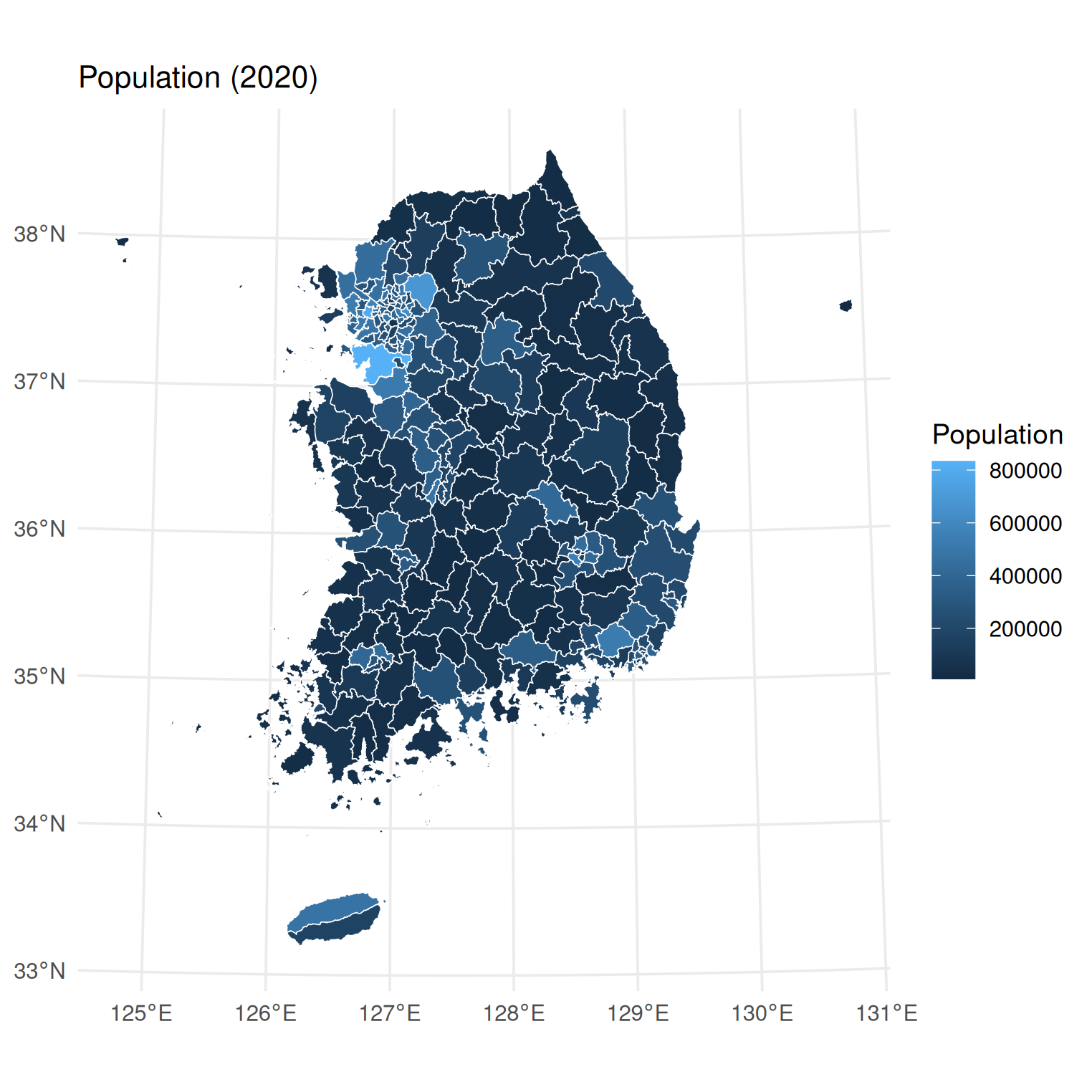
anycensus() will return an analysis-ready data.frame that can be easily merged with the corresponding boundary sf object from load_districts(). Here is a simple example of making maps with population data.
library(tidycensuskr)
#> tidycensuskr 0.2.7 (2026-02-26)
#> Please install the companion data package tidycensuskr.sf to use the district boundaries.
#> install.packages('tidycensuskr.sf', repos = 'https://sigmafelix.r-universe.dev')
library(ggplot2)
library(dplyr)
#>
#> Attaching package: 'dplyr'
#> The following objects are masked from 'package:stats':
#>
#>     filter, lag
#> The following objects are masked from 'package:base':
#>
#>     intersect, setdiff, setequal, union
library(tidyr)
library(sf)
#> Linking to GEOS 3.12.1, GDAL 3.8.4, PROJ 9.4.0; sf_use_s2() is TRUE
library(biscale)
library(cowplot)
sf_use_s2(FALSE)
#> Spherical geometry (s2) switched off
options(scipen = 100)

# load census data
census_pop_2020 <- anycensus(year = 2020, codes = NULL, type = "population")
#> Using character codes that are convertible to integers. Automatically converting to integers...
census_pop_2020 <- census_pop_2020 |>
  rename(population_total = `all households_total_prs`)

# load boundaries
data(adm2_sf_2020)
adm2_2020 <- adm2_sf_2020

# merge boundaries and census data
census_2020_sf <- adm2_2020 |>
  left_join(census_pop_2020, by = c("adm2_code" = "adm2_code"))

# plot population data
census_2020_pop <-
  ggplot(census_2020_sf) +
  geom_sf(aes(fill = population_total), color = "white", size = 0.1) +
  theme_minimal() +
  labs(
    title = "Population (2020)",
    fill = "Population"
  ) +
  theme(
    plot.title = element_text(size = 12),
    axis.text = element_text(size = 7),
    legend.text = element_text(size = 7),
    legend.title = element_text(size = 8)
  )

census_2020_pop
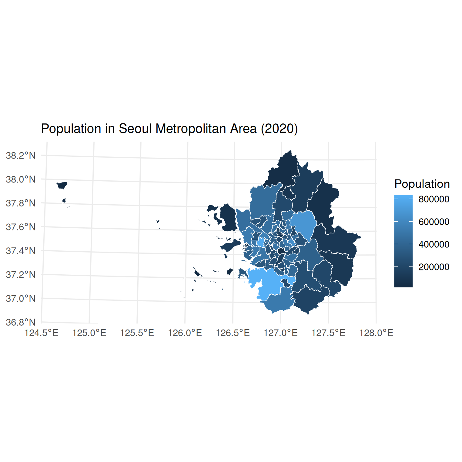
For Seoul Metropolitan Area (including Seoul, Incheon, and Gyeonggi-do), you can use a character vector in codes argument and merge the retrieved data.frame and sf object with inner_join():
census_pop_2020_sma <-
  anycensus(
    year = 2020,
    codes = c("Seoul", "Incheon", "Gyeonggi"),
    type = "population"
  ) |>
  rename(population_total = `all households_total_prs`)

census_2020_sf_sma <- adm2_2020 |>
  inner_join(census_pop_2020_sma, by = c("year", "adm2_code"))


# plot population data
census_2020_pop_sma <-
  ggplot(census_2020_sf_sma) +
  geom_sf(aes(fill = population_total), color = "white", size = 0.1) +
  theme_minimal() +
  labs(
    title = "Population in Seoul Metropolitan Area (2020)",
    fill = "Population"
  ) +
  theme(
    plot.title = element_text(size = 12),
    axis.text = element_text(size = 7),
    legend.text = element_text(size = 7),
    legend.title = element_text(size = 8)
  )

census_2020_pop_sma
Bivariate map
Moving on to a complex example, the code below demonstrates to generate a bivariate map with persons per housing unit and all-cause mortality rate.
census_housing_2020 <- anycensus(year = 2020, codes = NULL, type = "housing")
#> Using character codes that are convertible to integers. Automatically converting to integers...
census_housing_2020 <- census_housing_2020 |>
  rename(housing_total_units = `housing types_total_cnt`)
census_pop_housing_2020 <- census_pop_2020 |>
  left_join(
    census_housing_2020 |>
      select(adm2_code, housing_total_units),
    by = "adm2_code"
  ) |>
  transmute(
    adm2_code = adm2_code,
    persons_per_housing = population_total / housing_total_units
  )
census_mort_2020 <- anycensus(year = 2020, codes = NULL, type = "mortality")
#> Using character codes that are convertible to integers. Automatically converting to integers...
census_mort_2020 <- census_mort_2020 |>
  rename(mortality_total = `all causes_total_p1p`)

census_pph_mort_2020 <- census_pop_housing_2020 |>
  left_join(
    census_mort_2020 |>
      select(adm2_code, mortality_total),
    by = "adm2_code"
  )

# merge boundaries and census data
census_2020_sf <- adm2_2020 |>
  left_join(census_pph_mort_2020, by = c("adm2_code" = "adm2_code"))
census_2020_mapbase <-
  biscale::bi_class(
    census_2020_sf,
    x = persons_per_housing,
    y = mortality_total,
    style = "quantile",
    dim = 3
  )

# draw a bivariate legend
legend <- bi_legend(
  pal = "DkCyan",
  dim = 3,
  xlab = "More Persons per Housing ",
  ylab = "All-Cause Mortality ",
  size = 6
)

# plot population data
census_2020_bmap <-
  ggplot(census_2020_mapbase) +
  geom_sf(
    aes(fill = bi_class),
    color = "white",
    size = 0.1,
    show.legend = FALSE
  ) +
  bi_scale_fill(pal = "DkCyan", dim = 3) +
  theme_minimal() +
  labs(title = "Persons per housing unit and all-cause mortality rate (2020)") +
  bi_theme(base_size = 10) +
  theme(plot.title = element_text(size = 10))

# combine map with legend
census_2020_bimap <- cowplot::ggdraw() +
  cowplot::draw_plot(census_2020_bmap, 0, 0, 1, 1) +
  cowplot::draw_plot(legend, 0.7, 0.02, 0.3, 0.3)


census_2020_bimap
