Analytics Gallery with tidycensuskr

September 23, 2025

Example 1: Spatial autocorrelation of economic activity in South Korea

Design idea

In this example, we use Moran’s I statistics to analyze the spatial distribution of economic activity (measured by the number of registered companies) across South Korea in 2020.

• Global Moran’s I evaluates whether there is overall spatial autocorrelation, i.e., whether areas with similar company counts tend to cluster together nationwide.
• Local Moran’s I (LISA) identifies local clusters and outliers by classifying each district into four types:
  • High–High (H–H): districts with high values surrounded by other high-value districts.
  • Low–Low (L–L): districts with low values surrounded by other low-value districts.
  • High–Low (H–L): potential spatial outliers with high values surrounded by low-value neighbors.
  • Low–High (L–H): potential spatial outliers with low values surrounded by high-value neighbors.

The resulting LISA cluster map highlights where economic activities are concentrated and where they are sparse relative to neighboring areas.

Data prep

# Load 2020 boundaries
sf_2020 <- load_districts(year = 2020)

# Load 2020 economy data
df_2020_economy <- anycensus(year = 2020, 
                             type = "economy")

# Merge with spatial data
sf_2020_economy <- sf_2020 |>
  inner_join(df_2020_economy, by = "adm2_code") 

# Variable of interest: number of companies
var <- sf_2020_economy$company_total_cnt

Global Moran’s I

# Build neighbors (queen contiguity) and spatial weights
nb <- poly2nb(sf_2020_economy, queen = TRUE)
lw <- nb2listw(nb, style = "W", zero.policy = TRUE)

# Global Moran's I test
global_moran <- moran.test(var, lw, zero.policy = TRUE)
global_moran

## 
##  Moran I test under randomisation
## 
## data:  var  
## weights: lw  
## n reduced by no-neighbour observations  
## 
## Moran I statistic standard deviate = 10.35, p-value < 2.2e-16
## alternative hypothesis: greater
## sample estimates:
## Moran I statistic       Expectation          Variance 
##       0.424571643      -0.004149378       0.001715960

Local Moran’s I and LISA map

# Local Moran’s I
local_moran <- localmoran(var, lw, zero.policy = TRUE)

# Bind results back to sf object
sf_2020_economy <- sf_2020_economy |>
  mutate(
    Ii   = local_moran[, "Ii"],
    pval = local_moran[, "Pr(z != E(Ii))"]
  )

mean_var <- mean(var, na.rm = TRUE)

sf_2020_economy <- sf_2020_economy |>
  mutate(
    cluster = case_when(
      var > mean_var & Ii > 0 & pval <= 0.05 ~ "High-High",
      var < mean_var & Ii > 0 & pval <= 0.05 ~ "Low-Low",
      var > mean_var & Ii < 0 & pval <= 0.05 ~ "High-Low",
      var < mean_var & Ii < 0 & pval <= 0.05 ~ "Low-High",
      TRUE ~ "Not significant"
    )
  )

ggplot(sf_2020_economy) +
  geom_sf(aes(fill = cluster), color = "grey70", size = 0.05) +
  scale_fill_manual(
    values = c(
      "High-High"     = "red",
      "Low-Low"       = "blue",
      "High-Low"      = "pink",
      "Low-High"      = "lightblue",
      "Not significant" = "white"
    )
  ) +
  labs(title = "LISA Cluster Map of Company units (2020)") +
  theme_minimal()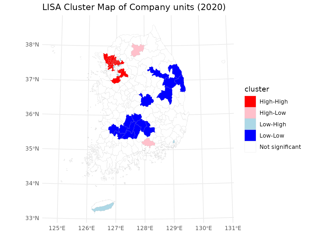

The results reveal a strong metropolitan concentration of economic activity. High–High (H–H) clusters are predominantly located in the Seoul Metropolitan Area, reflecting its central role in South Korea’s economy. Low–Low (L–L) clusters appear in Gangwon Province and along the borders of Jeollabuk-do, Jeollanam-do, Gyeongsangbuk-do, and Chungcheongnam-do, indicating regions with consistently low levels of company presence. This spatial pattern highlights the dominance of the capital region in economic activity and the relative sparsity of industrial and business units in peripheral provinces.