Getting Started with tidycensuskr
The tidycensuskr package provides easy access to South
Korean census and socioeconomic statistics, along with corresponding
geospatial boundary data. With this package, R users can query and
visualize population, housing, economy, tax, and mortality data linked
to administrative districts.
Load the package:
tidycensuskr will work at its full potential with the companion data
package tidycensuskr.sf, which contains the district
boundaries of South Korea. The package can be installed from
R-universe:
install.packages("tidycensuskr.sf", repos = "https://sigmafelix.r-universe.dev")After installing the companion package, three RDS files for 2010,
2015, and 2020 will be accessible through the function
system.file(). For example, the RDS file path of the 2010
district boundaries can be loaded as follows:
fs10 <- system.file("extdata", "adm2_sf_2010.rds", package = "tidycensuskr.sf")
adm2_sf_2010 <- readRDS(fs10)
1. Understanding Korean Geographic Hierarchies
South Korean census data is organized by three levels of administrative divisions:
-
Si-Do: The highest level of administrative
division.
- Metropolitan cities are treated as provinces.
- Jeju-do, Gangwon-do, and Jeollabuk-do have special self-governing status under Korean law.
-
Si-Gun-Gu: The second level, which
includes cities and counties.
- Si: Cities (urban administrative units)
- Gun: Counties (rural areas, typically <50,000 population)
-
Gu: Districts (urban subdivisions of
metropolitan cities or large cities).
- Gu under metropolitan cities are autonomous districts
- Gu under 11 large cities, as of 2025 (i.e., Suwon-si, Seongnam-si, Anyang-si, Goyang-si, Ansan-si, Yongin-si, Cheongju-si, Cheonan-si, Pohang-si, Changwon-si, Jeonju-si), are administraitve districts
-
Eup-Myeon-Dong: The third level, which
includes town and districts. (planned for future releases)
- Eup: Towns (urban, >20,000 population, within a county)
- Myeon: Townships (rural, <20,000 population, within a county)
- Dong: Neighborhoods (smallest units within cities and districts)
Comparison of Administrative Divisions
The table below provides a rough comparison of administrative divisions across South Korea, the United States, the European Union, and the United Kingdom (England). While the correspondence is not exact, it can be helpful to understand the approximate levels when working with census or regional data.
| South Korea | US | EU (NUTS1) | UK (England) |
|---|---|---|---|
| Si/Do | State | NUTS1 | Regions / Combined Authorities |
| Si/Gun/Gu | County | NUTS2 | County |
| Eup/Myeon/Dong | Townships / Towns / Census County Division | NUTS3 | Districts / Wards / Boroughs |

Because administrative boundaries and coding systems can vary across
years and data sources, tidycensuskr standardizes
administrative codes to allow consistent integration of statistics.
Currently, for 2020 data there are 250 Si-Gun-Gu and 17
Si-Do.
2. Available census data
The package provides census and survey data through:
- The function anycensus() for querying subsets
- The built-in dataset censuskor in long format
Data types
| type | class1 | class2 | unit | description | available |
|---|---|---|---|---|---|
| population | all households | total | persons | Total population count | 2010, 2015, 2020 |
| population | all households | male | persons | Male population count | 2010, 2015, 2020 |
| population | all households | female | persons | Female population count | 2010, 2015, 2020 |
| tax | income | general | million KRW | General income tax revenue | 2020 |
| tax | income | labor | million KRW | Labor income tax revenue | 2020 |
| mortality | All causes | total | per 100k population | Total mortality rate from all causes | 2020 |
| mortality | All causes | male | per 100k population | Male mortality rate from all causes | 2020 |
| mortality | All causes | female | per 100k population | Female mortality rate from all causes | 2020 |
| economy | company | total | count | Total number of companies | 2010, 2015, 2020 |
| housing | housing types | total | count | Total number of housing units | 2010, 2015, 2020 |
| housing | housing types | detached housing | count | Number of detached/single-family houses | 2010, 2015, 2020 |
| housing | housing types | apartment | count | Number of apartment units | 2010, 2015, 2020 |
| housing | housing types | row house | count | Number of row house units | 2010, 2015, 2020 |
| housing | housing types | multiplex | count | Number of multiplex housing units | 2010, 2015, 2020 |
| housing | housing types | non-residential | count | Number of non-residential buildings used for housing | 2010, 2015, 2020 |
| medicine | doctors | anesthesiology and pain medicine | persons | Number of anesthesiologists | 2010, 2015, 2020 |
| medicine | doctors | clinical laboratory medicine | persons | Number of clinical laboratory physicians | 2010, 2015, 2020 |
| medicine | doctors | dermatology | persons | Number of dermatologists | 2010, 2015, 2020 |
| medicine | doctors | emergency medicine | persons | Number of emergency medicine physicians | 2010, 2015, 2020 |
| medicine | doctors | family medicine | persons | Number of family medicine physicians | 2010, 2015, 2020 |
| medicine | doctors | internal medicine | persons | Number of internal medicine physicians | 2010, 2015, 2020 |
| medicine | doctors | neurology | persons | Number of neurologists | 2010, 2015, 2020 |
| medicine | doctors | neurosurgery | persons | Number of neurosurgeons | 2010, 2015, 2020 |
| medicine | doctors | nuclear medicine | persons | Number of nuclear medicine physicians | 2010, 2015, 2020 |
| medicine | doctors | obstetrics and gynecology | persons | Number of OB/GYN physicians | 2010, 2015, 2020 |
| medicine | doctors | occupational and environmental medicine | persons | Number of occupational/environmental medicine physicians | 2010, 2015, 2020 |
| medicine | doctors | ophthalmology | persons | Number of ophthalmologists | 2010, 2015, 2020 |
| medicine | doctors | orthopedics | persons | Number of orthopedic surgeons | 2010, 2015, 2020 |
| medicine | doctors | otorhinolaryngology | persons | Number of ENT specialists | 2010, 2015, 2020 |
| medicine | doctors | pathology | persons | Number of pathologists | 2010, 2015, 2020 |
| medicine | doctors | pediatrics | persons | Number of pediatricians | 2010, 2015, 2020 |
| medicine | doctors | plastic surgery | persons | Number of plastic surgeons | 2010, 2015, 2020 |
| medicine | doctors | preventive medicine | persons | Number of preventive medicine physicians | 2010, 2015, 2020 |
| medicine | doctors | psychiatry | persons | Number of psychiatrists | 2010, 2015, 2020 |
| medicine | doctors | radiation oncology | persons | Number of radiation oncologists | 2010, 2015, 2020 |
| medicine | doctors | radiology | persons | Number of radiologists | 2010, 2015, 2020 |
| medicine | doctors | rehabilitation medicine | persons | Number of rehabilitation medicine physicians | 2010, 2015, 2020 |
| medicine | doctors | surgery | persons | Number of general surgeons | 2010, 2015, 2020 |
| medicine | doctors | thoracic and cardiovascular surgery | persons | Number of thoracic/cardiovascular surgeons | 2010, 2015, 2020 |
| medicine | doctors | total | persons | Total number of doctors across all specialties | 2010, 2015, 2020 |
| medicine | doctors | tuberculosis | persons | Number of tuberculosis specialists | 2010, 2015, 2020 |
| medicine | doctors | urology | persons | Number of urologists | 2010, 2015, 2020 |
| migration | marital | female | count | Number of female marriage migrants | 2010, 2015, 2020 |
| migration | marital | male | count | Number of male marriage migrants | 2010, 2015, 2020 |
| migration | marital | total | count | Total number of marriage migrants | 2010, 2015, 2020 |
| environment | organic_matter | discharge | kg_day | Daily organic matter discharge | 2010, 2015, 2020 |
| environment | wastewater | generation | m3_day | Daily wastewater generation volume | 2010, 2015, 2020 |
| environment | wastewater | discharge | m3_day | Daily wastewater discharge volume | 2010, 2015, 2020 |
| environment | organic_matter | generation | kg_day | Daily organic matter generation | 2010, 2015, 2020 |
| population | fertility | total | births | Total number of births | 2010, 2015, 2020 |
| population | fertility | 15-19 (simulated) | births per 1000 | Age-specific fertility rate for ages 15-19 (simulated) | 2010, 2015, 2020 |
| population | fertility | 20-24 | births per 1000 | Age-specific fertility rate for ages 20-24 | 2010, 2015, 2020 |
| population | fertility | 25-29 | births per 1000 | Age-specific fertility rate for ages 25-29 | 2010, 2015, 2020 |
| population | fertility | 30-34 | births per 1000 | Age-specific fertility rate for ages 30-34 | 2010, 2015, 2020 |
| population | fertility | 35-39 | births per 1000 | Age-specific fertility rate for ages 35-39 | 2010, 2015, 2020 |
| population | fertility | 40-44 | births per 1000 | Age-specific fertility rate for ages 40-44 | 2010, 2015, 2020 |
| population | fertility | 45-49 | births per 1000 | Age-specific fertility rate for ages 45-49 | 2010, 2015, 2020 |
| economy | grdp | gross regional domestic product at market prices | million KRW | Total GRDP at market prices | 2010, 2015, 2020 |
| economy | grdp | net taxes on products | million KRW | Net taxes on products component of GRDP | 2010, 2015, 2020 |
| economy | grdp | total value added at basic prices | million KRW | Total value added at basic prices | 2010, 2015, 2020 |
| economy | grdp | agriculture, forestry and fishing | million KRW | GRDP from agriculture, forestry, and fishing sector | 2010, 2015, 2020 |
| economy | grdp | mining and quarrying | million KRW | GRDP from mining and quarrying sector | 2010, 2015, 2020 |
| economy | grdp | manufacturing | million KRW | GRDP from manufacturing sector | 2010, 2015, 2020 |
| economy | grdp | electricity, gas, steam and air conditioning supply; water supply and waste management | million KRW | GRDP from utilities and waste management sector | 2010, 2015, 2020 |
| economy | grdp | construction | million KRW | GRDP from construction sector | 2010, 2015, 2020 |
| economy | grdp | wholesale and retail trade | million KRW | GRDP from wholesale and retail trade sector | 2010, 2015, 2020 |
| economy | grdp | transportation and storage | million KRW | GRDP from transportation and storage sector | 2010, 2015, 2020 |
| economy | grdp | accommodation and food service activities | million KRW | GRDP from accommodation and food services sector | 2010, 2015, 2020 |
| economy | grdp | information and communication | million KRW | GRDP from information and communication sector | 2010, 2015, 2020 |
| economy | grdp | financial and insurance activities | million KRW | GRDP from financial and insurance sector | 2010, 2015, 2020 |
| economy | grdp | real estate activities; rental and leasing activities | million KRW | GRDP from real estate and rental sector | 2010, 2015, 2020 |
| economy | grdp | professional, scientific and technical activities; business support facilities | million KRW | GRDP from professional/technical services sector | 2010, 2015, 2020 |
| economy | grdp | public administration and defence; compulsory social security | million KRW | GRDP from public administration sector | 2010, 2015, 2020 |
| economy | grdp | education | million KRW | GRDP from education sector | 2010, 2015, 2020 |
| economy | grdp | human health and social work activities | million KRW | GRDP from health and social work sector | 2010, 2015, 2020 |
| economy | grdp | arts, sports and recreation; membership organizations and personal services | million KRW | GRDP from arts, recreation, and personal services sector | 2010, 2015, 2020 |
| social security | basic living security | female | persons | Female recipients of basic living security benefits | 2010, 2015, 2020 |
| social security | basic living security | male | persons | Male recipients of basic living security benefits | 2010, 2015, 2020 |
| social security | basic pension | male | persons | Male recipients of basic pension | 2015, 2020 |
| social security | basic pension | female | persons | Female recipients of basic pension | 2015, 2020 |
| welfare | facilities | residential facility | count | Number of residential welfare facilities | 2015, 2020 |
| welfare | facilities | service facility | count | Number of service-oriented welfare facilities | 2015, 2020 |
| welfare | facilities | other facility | count | Number of other welfare facilities | 2015, 2020 |
| welfare | registered physically mentally challenged | female_0-19 | persons | Registered disabled females aged 0-19 | 2015, 2020 |
| welfare | registered physically mentally challenged | female_20-39 | persons | Registered disabled females aged 20-39 | 2015, 2020 |
| welfare | registered physically mentally challenged | female_40-64 | persons | Registered disabled females aged 40-64 | 2015, 2020 |
| welfare | registered physically mentally challenged | female_65-79 | persons | Registered disabled females aged 65-79 | 2015, 2020 |
| welfare | registered physically mentally challenged | female_80+ | persons | Registered disabled females aged 80 and above | 2015, 2020 |
| welfare | registered physically mentally challenged | male_0-19 | persons | Registered disabled males aged 0-19 | 2015, 2020 |
| welfare | registered physically mentally challenged | male_20-39 | persons | Registered disabled males aged 20-39 | 2015, 2020 |
| welfare | registered physically mentally challenged | male_40-64 | persons | Registered disabled males aged 40-64 | 2015, 2020 |
| welfare | registered physically mentally challenged | male_65-79 | persons | Registered disabled males aged 65-79 | 2015, 2020 |
| welfare | registered physically mentally challenged | male_80+ | persons | Registered disabled males aged 80 and above | 2015, 2020 |
| welfare | registered physically mentally challenged severity | _0-19 | persons | Total registered disabled persons aged 0-19 | 2015 |
| welfare | registered physically mentally challenged severity | _20-39 | persons | Total registered disabled persons aged 20-39 | 2015 |
| welfare | registered physically mentally challenged severity | _40-64 | persons | Total registered disabled persons aged 40-64 | 2015 |
| welfare | registered physically mentally challenged severity | _65-79 | persons | Total registered disabled persons aged 65-79 | 2015 |
| welfare | registered physically mentally challenged severity | _80+ | persons | Total registered disabled persons aged 80 and above | 2015 |
| welfare | registered physically mentally challenged severity | less severely impaired_0-19 | persons | Less severely impaired persons aged 0-19 | 2020 |
| welfare | registered physically mentally challenged severity | less severely impaired_20-39 | persons | Less severely impaired persons aged 20-39 | 2020 |
| welfare | registered physically mentally challenged severity | less severely impaired_40-64 | persons | Less severely impaired persons aged 40-64 | 2020 |
| welfare | registered physically mentally challenged severity | less severely impaired_65-79 | persons | Less severely impaired persons aged 65-79 | 2020 |
| welfare | registered physically mentally challenged severity | less severely impaired_80+ | persons | Less severely impaired persons aged 80 and above | 2020 |
| welfare | registered physically mentally challenged severity | severely impaired_0-19 | persons | Severely impaired persons aged 0-19 | 2020 |
| welfare | registered physically mentally challenged severity | severely impaired_20-39 | persons | Severely impaired persons aged 20-39 | 2020 |
| welfare | registered physically mentally challenged severity | severely impaired_40-64 | persons | Severely impaired persons aged 40-64 | 2020 |
| welfare | registered physically mentally challenged severity | severely impaired_65-79 | persons | Severely impaired persons aged 65-79 | 2020 |
| welfare | registered physically mentally challenged severity | severely impaired_80+ | persons | Severely impaired persons aged 80 and above | 2020 |
| housing | vacant housing | fraction | percent | Percentage of vacant housing units | 2015, 2020 |
| housing | vacant housing | number of vacant housing | count | Total number of vacant housing units | 2015, 2020 |
| housing | vacant housing | total number of housing | count | Total number of housing units (occupied and vacant) | 2015, 2020 |
| landuse | greenspace | number of greenspace | count | Number of greenspaces | 2010, 2015, 2020 |
| landuse | greenspace | area of greenspace | square meters | Total area of greenspaces | 2010, 2015, 2020 |
| landuse | parks | number of parks | count | Number of parks | 2010, 2015, 2020 |
| landuse | parks | area of parks | square meters | Total area of parks | 2010, 2015, 2020 |
| landuse | road | length of roads | meters | Total length of roads | 2010, 2015, 2020 |
| landuse | road | area of roads | square meters | Total area of roads | 2010, 2015, 2020 |
Query data using anycensus()
The function anycensus() returns a tidy tibble with
columns such as:
-
year: year of the dataset -
adm1,adm1_code: Si-Do (province) level administrative unit name and its corresponding code -
adm2,adm2_code: Si-Gun-Gu (district) level administrative unit name and its corresponding code
Columns containing the values are added as a wide form. The column
adm2_code links census data directly to boundary files
retrieved with load_districts().
df_2020 <- anycensus(year = 2020,
                     type = "mortality",
                     level = "adm2")
head(df_2020)
#> # A tibble: 6 × 9
#>    year adm1              adm1_code adm2  adm2_code type  `all causes_total_p1p`
#>   <dbl> <chr>                 <dbl> <chr>     <dbl> <chr>                  <dbl>
#> 1  2020 Chungcheongbuk-do        33 Cheo…     33040 mort…                   312.
#> 2  2020 Chungcheongnam-do        34 Cheo…     34010 mort…                   321.
#> 3  2020 Gyeongsangbuk-do         37 Poha…     37010 mort…                   318.
#> 4  2020 Gyeongsangnam-do         38 Chan…     38110 mort…                   323.
#> 5  2020 Jeollabuk-do             35 Jeon…     35010 mort…                   283.
#> 6  2020 Gyeongsangbuk-do         37 Ando…     37040 mort…                   353
#> # ℹ 2 more variables: `all causes_male_p1p` <dbl>,
#> #   `all causes_female_p1p` <dbl>
The function can also aggregate values to higher administrative
units. By specifying level = "adm1" and providing an
aggregation function, we obtain province-level (adm1)
results that summarize across all districts.
df_2020_sido <- anycensus(year = 2020,
                          type = "mortality",
                          level = "adm1",
                          aggregator = mean,
                          na.rm = TRUE)
head(df_2020_sido)
#> # A tibble: 6 × 7
#> # Groups:   year, type, adm1, adm1_code [6]
#>    year type      adm1    adm1_code `all causes_total_p1p` `all causes_male_p1p`
#>   <dbl> <chr>     <chr>       <dbl>                  <dbl>                 <dbl>
#> 1  2020 mortality Busan          21                   335.                  458.
#> 2  2020 mortality Chungc…        33                   344.                  469.
#> 3  2020 mortality Chungc…        34                   336.                  450.
#> 4  2020 mortality Daegu          22                   311.                  426.
#> 5  2020 mortality Daejeon        25                   306.                  399.
#> 6  2020 mortality Gangwo…        32                   340.                  466.
#> # ℹ 1 more variable: `all causes_female_p1p` <dbl>
Built-in dataset censuskor
You can access the whole dataset directly using the function
data(censuskor) which returns the built-in dataset in a
long form.
-
year: year of the dataset -
adm1,adm1_code: Si-Do (province) level administrative unit name and its corresponding code
-
adm2,adm2_code: Si-Gun-Gu (district) level administrative unit name and its corresponding code -
type: Types of census or survey -
class1,class2: Classification variables providing further breakdowns -
unit: Measurement unit for the value -
value: The observed census value for the given combination of year, region, and category
data(censuskor)
head(censuskor)
#> # A data frame: 6 × 10
#>    year adm1          adm1_code adm2  adm2_code type  class1 class2 unit   value
#> * <dbl> <chr>             <dbl> <chr>     <dbl> <chr> <chr>  <chr>  <chr>  <dbl>
#> 1  2010 Chungcheongb…        33 Cheo…     33010 popu… all h… total  pers… 646939
#> 2  2010 Chungcheongb…        33 Cheo…     33010 popu… all h… male   pers… 318355
#> 3  2010 Chungcheongb…        33 Cheo…     33010 popu… all h… female pers… 328584
#> 4  2020 Chungcheongb…        33 Cheo…     33040 tax   income gener… mill… 524478
#> 5  2020 Chungcheongb…        33 Cheo…     33040 tax   income labor  mill… 598560
#> 6  2015 Chungcheongb…        33 Cheo…     33040 popu… all h… total  pers… 797099
Quick Visualization
Since anycensus() returns tidy data, visualization with
ggplot2 is straightforward.
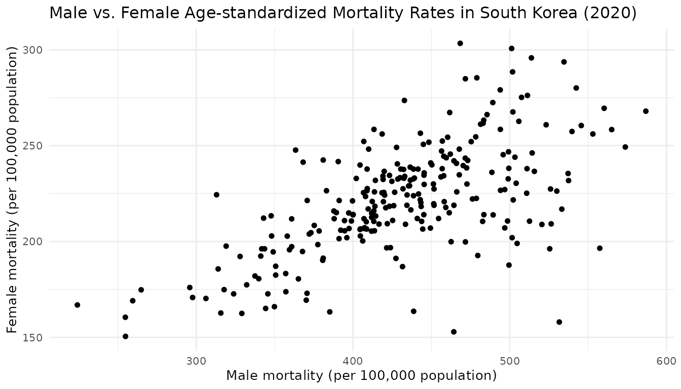
ggplot(df_2020, aes(x = `all causes_male_p1p`, y = `all causes_female_p1p`)) +
  geom_point() +
  labs(
    x = "Male mortality (per 100,000 population)",
    y = "Female mortality (per 100,000 population)",
    title = "Male vs. Female Age-standardized Mortality Rates in South Korea (2020)"
  ) +
  theme_minimal(base_size = 10)