예제 1: 한국 경제 활동의 공간적 자기상관
설계 아이디어
이 예제에서는 모란 I 통계량을 사용하여 2020년 한국의 경제 활동의 공간적 분포를 분석합니다. 경제 활동 지표는 시군구 별 사업체 수로 측정합니다.
- 전역적 모란 I 지수는 전체적인 공간적 자기상관이 존재하는지, 즉 기업 수가 비슷한 지역들이 전국적으로 뭉쳐 있는 경향이 있는지를 평가합니다.
- 국지적 모란 I 지수 (또는 국지적 자기상관지표, LISA)는 각
구역을 네 가지 유형으로 분류하여 국지적인 군집과 이상치를 식별합니다:
- 높음-높음 (H-H): 높은 값을 가진 구역이 다른 높은 값을 가진 구역들로 둘러싸인 경우.
- 낮음-낮음 (L-L): 낮은 값을 가진 구역이 다른 낮은 값을 가진 구역들로 둘러싸인 경우.
- 높음-낮음 (H-L): 높은 값을 가졌으나 낮은 값을 가진 이웃들로 둘러싸인 잠재적 공간 이상치.
- 낮음-높음 (L-H): 낮은 값을 가졌으나 높은 값을 가진 이웃들로 둘러싸인 잠재적 공간 이상치.
결과로 얻어지는 LISA 군집 지도는 주변 지역에 비해 경제 활동이 집중된 곳과 희소한 곳을 강조합니다.
데이터 준비
# Load 2020 boundaries
data(adm2_sf_2020)

# Load 2020 economy data
df_2020_economy <- anycensus(
  year = 2020,
  type = "economy"
)

# Merge with spatial data
adm2_sf_2020_economy <- adm2_sf_2020 |>
  dplyr::inner_join(df_2020_economy, by = "adm2_code")

# Variable of interest: number of companies
var <- adm2_sf_2020_economy$company_total_cnt
전역적(Global) Moran’s I
# Build neighbors (queen contiguity) and spatial weights
nb <- poly2nb(adm2_sf_2020_economy, queen = TRUE)
lw <- nb2listw(nb, style = "W", zero.policy = TRUE)

# Global Moran's I test
global_moran <- moran.test(var, lw, zero.policy = TRUE)
global_moran
##
## Moran I test under randomisation
##
## data: var
## weights: lw
## n reduced by no-neighbour observations
##
## Moran I statistic standard deviate = 10.35, p-value < 2.2e-16
## alternative hypothesis: greater
## sample estimates:
## Moran I statistic Expectation Variance
## 0.424571643 -0.004149378 0.001715960국지적(Local) Moran’s I 및 LISA 지도
# Local Moran's I
local_moran <- localmoran(var, lw, zero.policy = TRUE)

# Bind results back to sf object
adm2_sf_2020_economy <- adm2_sf_2020_economy |>
  mutate(
    Ii   = local_moran[, "Ii"],
    pval = local_moran[, "Pr(z != E(Ii))"]
  )

mean_var <- mean(var, na.rm = TRUE)

adm2_sf_2020_economy <- adm2_sf_2020_economy |>
  mutate(
    cluster = case_when(
      var > mean_var & Ii > 0 & pval <= 0.05 ~ "High-High",
      var < mean_var & Ii > 0 & pval <= 0.05 ~ "Low-Low",
      var > mean_var & Ii < 0 & pval <= 0.05 ~ "High-Low",
      var < mean_var & Ii < 0 & pval <= 0.05 ~ "Low-High",
      TRUE ~ "Not significant"
    )
  )

ggplot(adm2_sf_2020_economy) +
  geom_sf(aes(fill = cluster), color = "grey70", size = 0.05) +
  scale_fill_manual(
    values = c(
      "High-High" = "red",
      "Low-Low" = "blue",
      "High-Low" = "pink",
      "Low-High" = "lightblue",
      "Not significant" = "white"
    )
  ) +
  labs(title = "LISA Cluster Map of Company units (2020)") +
  theme_minimal()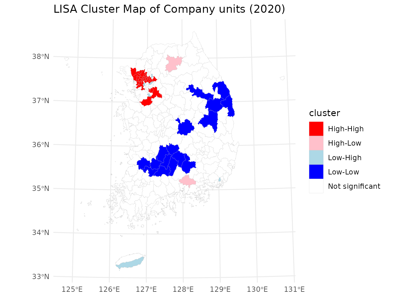
결과는 경제 활동이 고도로 수도권에 집중되어 있음을 보여줍니다. 높음-높음 (H-H) 군집은 주로 서울 수도권 지역에 위치하여 이 지역이 한국 경제에서 차지하는 중심적인 역할을 보여줍니다. 낮음-낮음 (L-L) 군집은 강원도와 전라북도, 전라남도, 경상북도, 충청남도의 경계 지역에 나타나며, 이는 기업 출현이 지속적으로 낮은 지역임을 나타냅니다. 이러한 공간적 패턴은 경제 활동에서의 수도권의 우위와 외곽 지역의 기업의 상대적 희소성을 반영합니다.
예제 2: 성별 및 지역별 인구 변화
설계 아이디어
-
tidycensuskr에 포함된censuskor데이터를 불러와 adm2 레벨의 성별 인구수에 집중합니다. - 시간이 지남에 따른 지역명 변경, 승격, 경계 조정을 반영하여 행정 구역 코드를 정리하고 정렬합니다.
- 인구수를 비교 가능한 단위(천 명)로 변환하고 일관된 라벨링을 위해 가장 최근의 지역명을 유지합니다. 중복 지역명 (예, 남구, 서구, 고성군 등)을 구분하기 위해 시군구 이름을 시도 약칭을 붙인 이름으로 재구성합니다.
- 2020년 행정 구역 경계를 기반으로
geofacet그리드를 준비합니다. - 남성과 여성의 인구 추세를 선형 차트를 사용하여 중첩 시각화합니다.
# load packages
library(geofacet)

# load bundled data in tidycensuskr
data(censuskor)
data(adm2_sf_2020)
data(kr_grid_adm2_sgis_2020)

# prepare geofacet grid data
# Use the newest adm2_code and name if one got its name changed or promoted
pop <- censuskor |>
  dplyr::filter(
    type == "population" & class1 == "all households"
  ) |>
  dplyr::rename(code = adm2_code) |>
  dplyr::filter(class1 == "all households", class2 != "total") |>
  dplyr::mutate(
    value = value / 1000,
    code = dplyr::case_when(
      # Michuhol-gu (i.e., 23030 to 23090)
      code == 23030 ~ 23090,
      # Yeoju-si
      code == 31320 ~ 31280,
      # Dangjin-si
      code == 34390 ~ 34080,
      TRUE ~ code
    )
  ) |>
  dplyr::arrange(code, class2, -year) |>
  dplyr::group_by(code) |>
  dplyr::mutate(adm2 = adm2[which.max(year)]) |>
  dplyr::ungroup()

head(pop)
## # A tibble: 6 × 10
## year adm1 adm1_code adm2 code type class1 class2 unit value
## <dbl> <chr> <dbl> <chr> <dbl> <chr> <chr> <chr> <chr> <dbl>
## 1 2020 Seoul 11 Jongno-gu 11010 population all house… female pers… 72.6
## 2 2015 Seoul 11 Jongno-gu 11010 population all house… female pers… 73.8
## 3 2010 Seoul 11 Jongno-gu 11010 population all house… female pers… 76.5
## 4 2020 Seoul 11 Jongno-gu 11010 population all house… male pers… 67.3
## 5 2015 Seoul 11 Jongno-gu 11010 population all house… male pers… 69.5
## 6 2010 Seoul 11 Jongno-gu 11010 population all house… male pers… 71.3
# for a geofacet plot
# map codes to district names for facet labels
pop_name_map <- pop %>%
  dplyr::distinct(code, adm2) %>%
  {
    setNames(.$adm2, .$code)
  }

pop_labels <- pop %>% dplyr::distinct(code, adm2)

# Adjust for the identical district names in different provinces
kr_grid_adm2_sgis_2020 <-
  kr_grid_adm2_sgis_2020 |>
  dplyr::mutate(
    name = dplyr::case_when(
      grepl("^32", code) & name == "Goseong-gun" ~ "Goseong-gun (GW)",
      grepl("^38", code) & name == "Goseong-gun" ~ "Goseong-gun (GN)",
      grepl("^11", code) & name == "Jung-gu" ~ "Jung-gu (SE)",
      grepl("^21", code) & name == "Jung-gu" ~ "Jung-gu (BU)",
      grepl("^22", code) & name == "Jung-gu" ~ "Jung-gu (DG)",
      grepl("^23", code) & name == "Jung-gu" ~ "Jung-gu (IC)",
      grepl("^25", code) & name == "Jung-gu" ~ "Jung-gu (DJ)",
      grepl("^26", code) & name == "Jung-gu" ~ "Jung-gu (UL)",
      grepl("^21", code) & name == "Seo-gu" ~ "Seo-gu (BU)",
      grepl("^22", code) & name == "Seo-gu" ~ "Seo-gu (DG)",
      grepl("^23", code) & name == "Seo-gu" ~ "Seo-gu (IC)",
      grepl("^24", code) & name == "Seo-gu" ~ "Seo-gu (GJ)",
      grepl("^25", code) & name == "Seo-gu" ~ "Seo-gu (DJ)",
      grepl("^26", code) & name == "Seo-gu" ~ "Seo-gu (UL)",
      grepl("^21", code) & name == "Nam-gu" ~ "Nam-gu (BU)",
      grepl("^22", code) & name == "Nam-gu" ~ "Nam-gu (DG)",
      grepl("^24", code) & name == "Nam-gu" ~ "Nam-gu (GJ)",
      grepl("^26", code) & name == "Nam-gu" ~ "Nam-gu (UL)",
      grepl("^21", code) & name == "Dong-gu" ~ "Dong-gu (BU)",
      grepl("^22", code) & name == "Dong-gu" ~ "Dong-gu (DG)",
      grepl("^23", code) & name == "Dong-gu" ~ "Dong-gu (IC)",
      grepl("^24", code) & name == "Dong-gu" ~ "Dong-gu (GJ)",
      grepl("^25", code) & name == "Dong-gu" ~ "Dong-gu (DJ)",
      grepl("^26", code) & name == "Dong-gu" ~ "Dong-gu (UL)",
      grepl("^21", code) & name == "Buk-gu" ~ "Buk-gu (BU)",
      grepl("^22", code) & name == "Buk-gu" ~ "Buk-gu (DG)",
      grepl("^24", code) & name == "Buk-gu" ~ "Buk-gu (GJ)",
      grepl("^26", code) & name == "Buk-gu" ~ "Buk-gu (UL)",
      grepl("^11", code) & name == "Gangseo-gu" ~ "Gangseo-gu (SE)",
      grepl("^21", code) & name == "Gangseo-gu" ~ "Gangseo-gu (BU)",
      TRUE ~ name
    )
  )
스몰 멀티플(Small multiples)
이 디자인은 각 시군구의 상대적 위치를 반영하는 공간 구조를 최대한 유지하면서 이질적인 지역 인구 변화 추이를 강조합니다.
ggplot(data = pop) +
  geom_line(
    aes(x = year, y = value, group = interaction(adm2, class2), color = class2),
    alpha = 0.5,
    linewidth = 1.5
  ) +
  facet_geo(~code, grid = kr_grid_adm2_sgis_2020, label = "name", scale = "free_y") +
  labs(
    title = "Population Trends in South Korea by Sex and District",
    x = "Year",
    y = "",
    color = "Population Class",
    caption = "Y-axis values are not commensurate with the original scale"
  ) +
  scale_color_manual(values = c(female = "#F44336", male = "#2196F3")) +
  theme_void() +
  scale_x_continuous(
    breaks = sort(unique(pop$year)),
    labels = function(x) sprintf("%d", as.integer(x))
  ) +
  theme(
    strip.text = element_text(
      size = 5,
      margin = margin(0.05, 0.05, 0.05, 0.05, "cm")
    ),
    strip.background = element_blank(),
    axis.text.x = element_text(size = 6, angle = 90, hjust = 1),
    axis.text.y = element_blank(),
    panel.spacing = grid::unit(1, "pt"),
    plot.margin = margin(1, 1, 1, 1, "mm")
  )